Surface Feature Detection using Laser Profile Scanners

Thesis

Sam Mathunny Kochukalikkal

943011565

Fifth Year Engineering Student – Computer Option

Academic Supervisor – Jacque Vaisey

Technical Supervisor – Jan Brdicko

Committee Member – Kamal Gupta

Table of Content

ABSTRACT..................................................................................................................................... .ii

ACKNOWLEDGEMENTS........ .........................................................................................................iii

GLOSSARY..................................................................................................................................... iv

LIST OF TABLES AND FIGURES......................................................................................................vii

1         INTRODUCTION......................................................................................................................1

1.1        Design Specifications.............................................................................................................1

1.2        Description & Background.......................................................................................................1

1.2.1             Bucking.........................................................................................................................2

1.2.2            Log Breakdown................................................................................................................2

1.2.3            Cant Sawing....................................................................................................................3   

1.2.4             Edging...........................................................................................................................3

1.2.5             Trimming........................................................................................................................3

1.2.6             Sorting and Packaging.............................................................................................3

1.3         Imaging Techniques....................................................................................................3

1.3.1             Speed of Operation.................................................................................................3

1.3.2             Image-Processing Techniques.....................................................................................3

1.3.3             Description of the two Scanners...................................................................................4

1.4        Error Analysis...............................................................................................................5

2         TECHNICAL CHALLENGES AND LIMITATIONS...........................................................................7

2.1        Data Capture................................................................................................................7

2.1.1             Scanner Head System................................................................................................7

2.1.2             Coordinate Systems...................................................................................................8

2.1.3             Calibration...........................................................................................................9

2.2         Profile Creation............................................................................................................11

2.2.1             Current technique and it’s limitations............................................................................11

2.2.2             Proposed techniques................................................................................................14

2.3         Surface Roughness Detection..................................................................................................22

2.3.1             Current technique............................................................................................................22

2.3.2             Some Useful Definitions Related to Detection of Surface Features........................................22

2.3.3             Course of Action..............................................................................................................23

3         EXPERIMENTAL ANALYSIS......................................................................................................26

3.1        Bump-Depression threshold determination.................................................................................26

3.1.1             Length of moving average – Long and Short........................................................................26

3.2        Test case................................................................................................................................27

3.3       Discussion of Results...............................................................................................................33

3.4        Accuracy of Bump location and size...........................................................................................34

3.5        Runtime Reduction...................................................................................................................34

4         CONCLUSION............................................................................................................................36

5         REFERENCE.............................................................................................................................37

APPENDIX A.........................................................................................................................................38

A.1 Hermary Scanner.............................................................................................................................38

A.1.1 Reference Beam Projector..............................................................................................................38

A.1.2 Linear Imaging Camera...................................................................................................................38

A.1.3 Processor......................................................................................................................................38

A.1.4 Communication..............................................................................................................................38

A.1.5 Laser Symboling Principle...............................................................................................................40

A.2 Dynavision Scanner...........................................................................................................................41

A.2.1 Scanner Configuration.....................................................................................................................41

A.2.2 Scanner Operation.......................................................................................................................... 42

A.2.3 Laser Triangulation Principle.............................................................................................................42

Appendix B..............................................................................................................................................43

Appendix C - USER INTERFACE...............................................................................................................44

ABSTRACT

The sawmill industry spends large amounts of money, time and manpower to increase the efficiency of processing logs and to extract the most value from logs. To achieve this objective, sawmills used to rely on people at every stage of log processing, but in modern sawmills human interaction has been replaced by state of the art machinery that significantly increases the yield. The logs are processed in multiple stages to manufacture the finished product. Each processing stage has been improved through the ages in an effort to increase the productivity of the sawmill industry. One of the main operations included in log processing is scanning of logs. The purpose of scanning is to identify the characteristics of a particular log such as size, shape, color and water content. Presently little research is undertaken in the field of Log Surface Scanning and no established procedures exist to measure surface roughness. My thesis project involved scanning log surfaces with the objective to locating features that would qualify the log to be either of low or high quality. Two different models of laser scanner have been made available for this work. They are the Hermary scanner and the Dynavision scanner.

The scanning technique supported by each of these scanners is different. Hermary scanners rely on a unique Laser Symboling principle whereby the coordinates of a point on the object in sight are obtained using symbols projected on the object. Dynavision scanners rely on a conventional Laser Triangulation principle. Eventhough the Dynavision scanners are not tested enough to compare it's performance in relation to the Hermary scanners, the algorithm proposed for the surface detection feature can be used for the Dynavision scanner too. This thesis also describes the research algorithms capable of detecting surface features on a log.

                                                               *********

ACKNOWLEDGEMENTS

I would like to thank these people in helping me out with my thesis.

Harkesh Grewal – Data Networking

Jan Brdicko – Technical Supervisor

Rudolf Dimistriu – Windows/C++ programmer 

Robert Danzer - Windows/C++ programmer

Susan Stevenson – Communications Instructor

Jacques Vaisey – Academic Supervisor

*********

GLOSSARY

Flyte – Carriage placed on the conveyer chain to transport the log.

Frame Coordinate System (FCS) – Coordinate system with the conveyer belt as the origin.

Head Coordinate System (HCS) – Coordinate system for the each individual head.

Median Scan - Scan that is nearest to the specified distance along the length of the log.

Moving Average - An average of certain user specified length that travels along the log length. The average can be of the strip points along the length of the log or it can be the average of the data points in a slice to smooth the slice.

Polar Coordinate System (PCS) – Coordinate system similar to the FCS accept the origin is the axis of the log.

Profile - Cross-section or slice of the log at a certain z-value. A profile is comprised of scans from all 4 heads.

Scan - Series of data points at a certain z-value.

Strip - An average of all the data points in the wedge. Each slice or cross-section is converted into strips and the number of strips equals the number of wedges.

Wedge - A “pizza slice” wedge like part of a single log cross-section with a certain user specified angle.   This angle is the same for all wedges in the cross-section and the sum of these angles must equal 360 degrees.  All log cross-sections are divided into the same number of wedges.

                                                                               *********

1         INTRODUCTION

A regular saw mill produces huge quantities of finished lumber and wood products every day and a delay in any aspect of log processing can cause a significant decline in the company’s productivity. Extracting the highest dollar value from each log depends on the particular method chosen to cut boards from logs, which can be determined using Laser scanning systems and software optimizing applications

Scanning the log and creating a log profile is one of the most vital tasks of sawmill operation. If the scanning technique is accurate and reliable, then the sawmill can extract the most dollar value out of a log. The earlier the scanning process detects a defect in a log, the better the end solution. The ability to detect surface features helps mostly in grading, bucking, and pattern optimizing; however, the exisiting scanners do not do well at detecting "roughness" features such as bumps and depressions. MPM Research Inc. is currently developing a software application that create a "true shape" log image, and then utilize this image to determine the best pattern for the cutting the log. My project involved optimizing the existing laser scanning technology for enhanced detection of surface features by modifying the existing software algorithms. More specifically, the objectives of my thesis were to create a solution to detect surface features on the lumber and to implement the results on the Hermary scanners. The specifications and constraints for ths design are provided in the following section. The solution was also implemented on the Dynavision scanner, however a thorough performance analysis wasn’t undertaken on the Dynavision scanner in this case.

1.1      Design Specifications

The real time execution speed of the scanner server, which includes the surface detection software, should be under 2secs. The surface features that should be detected by the scanner server are the location and size of bumps and depressions of under 6in height and depth. The accuracy in location and size of the bumps and depressions should be around under 0.5in. However initial study of the scanners and their scanning technology have shown that for such accuracy in bump location and size the scanner hardware needs to be modified. Specifically, the scan rate has to be improved by three fold for acquiring such bump accuracies. At present the scan rate is at 10ms/scan. With the present scanners the best accuracy available for bump location and size is 2in. More details about the design specifications are provided in Sections 1.3 and 3.0

1.2      Description & Background

Trees meant for logging are first stripped of their branches. Stripping takes place even before the tree is transported to the mill and hence this operation is beyond the control of the mill personnel. The resulting log is on average 80 – 100ft long. These logs are transported to sawmills where they are placed sequentially on a conveyer belts. A few common operations present in every sawmill are bucking, sorting, log breakdown, cant sawing, edging and trimming.

1.2.1          Bucking

Once on the conveyer belt, the log is scanned and the dimensions are provided to the Bucking Optimizer. The optimizer builds up a crude log image and determines a number of bucking solutions. Each bucking solution involves crosscutting the log into shorter pieces depending on the criteria provided by the sawmill. This solution is called an optimum bucking solution. Taper and diameters at the extremes of the log are also taken into account when determining the bucking solutions.

1.2.2          Log Breakdown

Each of the small logs is scanned to measure its length and surface dimensions, and this information is transmitted to the log optimizer. The log optimizer creates an image of the scanned log and determines the highest number of optimally sized boards that can be produced from the log. Like the bucking optimizer, the log optimizer calculates thousands of solutions and the best solution is selected depending on user specifications. Each solution involves sawing the log into cants (squared off logs), sidepieces and boards, as shown in figure 1. Sometimes, to acquire a preferred solution, the log is rotated about its longitudinal axis; additional scanning is then required to confirm that the rotation of the log was performed correctly to establish the best cutting pattern.

In some sawmills, sorting precedes log breakdown. Usually sorting involves manual labor, but this process is also being mechanized.

1.1.1          Cant Sawing

Cants are further processed in the cant sawing machine center. The cant is scanned and appropriately positioned and sawn to make smaller cants and boards.

1.1.2          Edging

Flitches (small cants) are processed in a machine center called an edger.  The flitches are scanned, optimally positioned and then edged to create smoother lumber.

1.1.3          Trimming

The trimmer operation processes boards created in the primary breakdown, cant sawing, and edging operations. The boards are scanned and crosscut into finished lengths.

1.1.4          Sorting and Packaging

All the cants, boards and sidepieces are scanned and sorted into the appropriated bins. These finished products are then packaged and sent to the vendors. Size, length, and grade are taken into consideration while sorting.

1.2      Imaging Techniques

This section explains why current scanning techniques are inadequate and what’s needed to upgrade existing systems. Background on the scanners that will be used for surface roughness detection is also provided.

1.2.1          Speed of Operation

A typical saw mill runs at an average feed rate of 300ft/min so that a log passes through the scan view zone at approximately 60in/sec. To accurately determine the surface roughness of a log requires a scan at least every 0.25in of the log. These two rates set the minimum scan rate limit to no less than 10ms. The current industry standard in B.C. sawmills is approximately 30ms.

1.2.2          Image-Processing Techniques

Most current image-processing techniques are too complicated and slow to detect surface features with the speed needed for sawmill use. The lack of speed is largely due to the computationally intensive algorithms that are used to produce the image of the object. For example, when an image-processing unit scans a log by obtaining a snap shot of the entire log, the 3D log image produced is then unwrapped and projected onto a 2D plane using a transformation matrix that contain the position and orientation of the origin of the sawing machine’s frame of reference. The 2D image undergoes various algorithms necessary for the accurate detection of surface roughness features. The bottleneck, in terms of speed, is the time-required feature to project the 3D-image onto an X-Y plane- a step that is unnecessary if the log image is dealt with entirely in the 2D plane.

These constraints could be overcome with a faster processor or by introducing DSPs hardware, but these solutions would result in increased costs. Fot this project, the company wanted the present hardware modified, in software to create an optimum log image and to detect surface roughness features using this image.

1.2.3          Description of the two Scanners

The analysis performed on the Hermary scanner helps to identify the technical limitations that will apply to the creation of the surface roughness detection feature. The next two sections contain brief descriptions of the Hermary and the Dynavision scanners. Please note that a performance comparison between the two scanners was not undertaken due to unavailability of the Dynavision scanner. The reason for mentioning the Dynavision scanner in this thesis report is because the solution to the surface roughness feature detection problem was also implemented in the Dynavision scanner and the preliminary results indicated that the solution worked just as well as it did in the Hermary scanner.

1.2.3.1         Hermary Scanner

The Laser Profile Scanner model LPS-2016 is a fully integrated, co-planar scanning system designed to scan logs for optimal utilization in sawmill settings. The LPS-2016 generates a two-dimensional profile of the surface that intersects the scan plane. The data from all the LPS-2016 heads are combined in the host computer system to obtain the complete log profile.

Two physical communication interfaces are available on the LPS Scanner. These ports allow for communication either on an asynchronous serial channel as well as on an ethernet channel supporting TCP/IP protocol. The asynchronous serial ASCII interface is used for maintenance and diagnostics purposes as well as for programming the Internet address. Real time profile data from a multiple head scan zone system is available on the Ethernet interface. A Detailed description of the communication interface for scanner and the scanner server is given in Appendix A

Hermary Scanners work according to the laser symboling principle whereby the coordinates of a point on the object in sight are obtained using symbols projected on the object. The size and location of the symbol on the object determine the location of the point. The scan rate of the LPS-2016 scanner is 10ms/scan, and with feed rates of 300 feet/minute the profiles can be acquired at 0.6” intervals along the length of the object. The results obtained from an error analysis performed on the Hermary scanner system reveal that the average error distance between the theoretical point position, i.e., the point position determined by the scanner, and the actual point position is 0.030in. The standard deviation of this error is approximately 0.015in. However, the maximum difference in distance between the theoretical and actual points is 0.15in.

1.2.3.2         Dynavision Scanner

The Dynavision scanner system is among the latest instruments developed in the field of 3D scanning technology. The scanner functions in the same manner as the Hermary scanners in regards to organizing the data. The difference between the two scanners is the method used to obtain the data points. With feed rates of 300 feet/minute, profiles can be acquired at 1” intervals along the length of an object. Data is transmitted from the scanner heads to the associated In combination with fiber-optic transmitters and receiver, it provides high noise immunity and a bandwidth of 100Mbps. Data transmitted from each scanner head is received in its corresponding Dynavision TAXI_IP_RX Host Interface where it is stored in a buffer (FIFO) within the interface. The scanner server then reads data from the FIFO. Appendix A contains a detailed description of the communication interfaces between the scanner heads and the scanner server.

In relation to the Hermary scanners, the Dynavision scanner operates with 250 profile points per head as compared to 100 points presented by the Hermary scanner. The Dynavision Scanner uses laser triangulation technology for scanning, and incorporates a processor-per-head approach to data processing using high speed, embedded computers. A detailed description of the laser triangulation and the laser symboling process is given in Appendix A.

1.3      Error Analysis

Table 1 contains the results of the error analysis performed on both the scanners and on the calibration procedure to determine the total error in the location of the data points. The test was performed using a calibration jig. The calibration jig was placed at a predetermined location and scan data was obtained from ten consecutive scans. The data points from the ten consecutive scans were used to determine a least square line through the scan data points. This least square line equation was compared with the line equation provided by the scanner itself. This test was also performed on the Dynavision scanner. However the calibration jig for the Dynavision scanner is different from the calibration used for the Hermary scanner and the jigs cannot be exchanged between the two scanners because of the design of the jig.

The result of the error analysis performed on both the scanners help to clearly define some of the problems associated with the surface roughness detection feature. These results also help define the constraints on the surface roughness feature detection algorithm. For example, no solution will be more accurate than 0.055in since this limit is indirectly set by the scanner hardware. These results also show that the reliability of the bump and depression come into question when the outline of the bumps and depressions are above the 30 degree reliability zone of the scanner. However, in a 4-head scanner system, the scan data points from each scanner head often overlap and thus this reliability issue is not a serious problem.

2         TECHNICAL CHALLENGES AND LIMITATIONS

This chapter describes the problems associated with data capture and surface roughness detection and also provides solutions to these problems.

2.1      Data Capture

One of the most important processes performed by the scanner server is the capture of data points and creation of a profile using these data points. A profile, as mentioned in the glossary, is a cross-section slice of the log at a particular z-value; a profile is created using scans from all scanner heads in a system. The success of the surface roughness detection feature depends heavily on the accuracy of the profile. The scanner head system can be configured in many different arrangements.

2.1.1          Scanner Head System

A system comprising of 4 scanners, or scanner heads, is often called a 4-Head scanner system (see Figure 2). The figure illustrates the coordinate system of individual scanner heads and their relationship to the machine frame coordinate system. More details regarding the coordinate systems and their relationship with each other are explained in following section. Similarly a 6-Head scanner system operates with 6 scanners, or scanner heads. At present, surface roughness detection will only be incorporated in the 4-Head scanner system because creating a solution to all types of scanner head systems is beyond the scope of this thesis project and also because a 4-Head scanner system is the most widely used scanning configuration in the Sawmill industry. A scanner head system can have less than 4 scanner heads, however extensive software modifications to the scanner server would be required to detect surface roughness features because all four quadrants of the log are not covered and therefore the scanner head system cannot create a complete log image without some form of complex pattern recognition and pattern filling scheme. The current technique used for capturing the scan data points from the logs, i.e., the technique used in the industry at present, performs well for product fit but this technique is not adequate to detect surface roughness features. A detailed explanation of the current data capture technique is provided in the upcoming sections, along with the problems associated with the technique. The data points are transformed from one coordinate system to another and then a profile is created with these transformed data points.

2.1.2          Coordinate Systems

There are three different coordinate systems that accompany the scanner system. Each scanner head has it’s own Head Coordinate System (HCS). The x-axis for this coordinate system is perpendicular to the scanner heads origin and the y-axis is parallel to the scanner heads (see Figure 2). The second coordinate systems is called the Frame Coordinate System (FCS) with the origin, called the frame center, located usually at the conveyer belt that passes through the frame of the scanner system. This second coordinate system maps the scan data points produced by the scanner heads from the scanner plane to the machine plane. The data points are converted from the HCS to the FCS using the following calibration equations:

For origin of the position of the scanner head H1

where

–       X-coordinate value of the origin of the Frame Coordinate System

 -            Orientation angle of Scanner head 1 in reference to the Frame Coordinate System

 & -   Coordinate values of the scan data point in the Head Coordinate System

A coordinate system was needed by the surface roughness feature algorithm to determine the bumps and the depressions with reference to the log center rather than the machine frame (FCS) origin. The HCS cannot be used for determining the bumps and depressions since there is usually more than one scanner head and thus more than one HCS. The machine FCS would not apply since the machine frame is log oriented, making it difficult to identify the location of the bumps and depressions. Thus another coordinate system was introduced that looked at the log from the inside out; this coordinate system is the polar coordinate system (PCS). All the data points in the FCS are converted to the Polar Coordinate System (PCS) with the center of the log as the origin. The center of the log is determined by smoothing the log image and then applying a moving average filter to the image. A detailed description on how the center is determined is provided in section 2.2.2.1. These three coordinate systems are important for surface roughness detection and will be mentioned frequently throughout this report. The data points are converted from the FCS to the PCS using the equation similar to the ones above.

2.1.3          Calibration

Calibration ensures that the data points read by the scanner are converted accurately to the FCS. Some of the calibration techniques currently used are explained below.

2.1.3.1         Calibration Fixture – Star, Pipe, Ring

The calibration procedure currently uses a star shaped fixture for performing calibration. This fixture does not resemble a log and limits the reliability of the calibration because the fixture is hard to mount on the flyte, which is used to transport logs. The calibration procedure takes a significant amount of time because the mill personnel have to dismantle the flight and chains that carry the logs to place the star shaped fixture in the proper location with respect to the scanner frame. Also after the calibration is done the flights have to be placed back on the machine system, which introduces error in the scanner frame origin. A comparison of the degree of accuracy of the two calibration processes, i.e. calibrations with the start shaped fixture and machined pipe fixture, was performed and results were similar. A summary of the analysis is provided in the error analysis section, i.e., section 1.3.

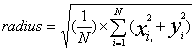
A machined pipe is the closest form to an actual log, and thus I have implemented a pipe calibration procedure that will supplement the star shaped fixture calibration. The pipe calibration uses a best-fit circle routine obtained from the Internet (Thomas Block, October 1999) for pattern matching. The routine uses the data points produced by scanning the machined pipe fixture to fit a circle with similar radius and center of the machined pipe. The input to the routine is the scan data points and the outputs are the radius and the center of the circle that fits within these scan data points.

2.1.3.2         Pipe Calibration

There are two methods of pipe calibration available for implementation. The first method uses only one pipe, however, this method depends on the mill personnel to provide accurate orientation angles of the heads. The second method uses two pipes and does not require the mill personnel to provide the orientation angles. In both methods, the user is asked for the pipe radius, pipe vertical and horizontal offset from the flyte. Both methods implement the best-fit circle routine, which reduces the error in the difference between each data point in the profile and the circumference of the circle that the best-fit circle routine produces. The best-fit circle routine calculates the radius and center of a circle that has the least error with the data points. The equations for the best-fit circle routine are given below:

Since the best fit circle routine uses the data points to determine a radius and a center it cannot be used to locate a center for a circle with radius, which we know as the pipe diameter is fixed. Therefore the initial center determined by the best-fit circle routine is the starting point for a search routine that locates the center for a circle of given radius that would fits in the scan data points. The search routine has a search span of twice the radius produced by the best-fit routine and a search increment of one-tenth the search span. Pseudo-code of the search routine is given in Appendix B.  A nested loop is used to narrow down the exact location of the center. The accuracy of the center is presently limited to 0.01in but in future can be lowered for greater accuracy.

 This procedure is implemented for both methods of pipe calibration. However, for two pipes calibration the routine uses the difference between the centers of the two pipes to extract the orientation angles of the heads provided by the mill personnel in the one pipe calibration. Both the calibration procedures, i.e., the calibration with the star shaped fixture and the machined pipe fixture were tested for comparison and the positions of the scanner heads were determined. Using the scanner head positions determined by calibration using the two fixtures, we found that the accuracy of the pipe calibration is as good as the star shaped fixture. However, it takes only 5min to perform the pipe calibration procedure, whereas it takes approximately 20min to perform the star shaped calibration procedure. With two pipes, the orientation of the angles are calculated internally by the scanner server, just as in the star shaped fixture calibration. However, I recommend that the difference in the pipe size be greater than 4 inches since there is an inverse-squared relationship between the difference in the pipe diameters and error in the calibration. For the calibration process, I used a 10in diameter pipe size and a 5in diameter pipe size.

2.2      Profile Creation

The issues related to the present profile creation method and the solutions to these issues are briefly explained below.

2.2.1          Current technique and it’s limitations

Profile, as mentioned above, is defined as a single cross-sectional slice of a log. A log image is comprisedof a set of these profiles. Scans from all four scanner heads (if it is a 4-Head scanner system) are merged together to create a profile. Improving the profile creation routine is important, since the surface roughness depends on the accuracy of the profile to the log. If the profile determined using the scan data points is not an accurate depiction of the cross section of the log, then the surface roughness algorithm will not function in an efficient manner. The flowchart in Figure 3 shows how data from the scanner heads passes through the different modules to eventually reach the PLC and the cut optimizer. The scanner server consists of three main modules; the input, the output and the processing module. The input of the scanner server is the data points from the scanner heads and the output is the instructions given to the PLC and the profile points given to the optimizer. All the functions in the input and processing modules have been modified to improve the profile creation technique. There were very few modifications to the output module. The next sub-sections explain the functions of the three modules.

2.2.1.1         Input - LPSThread

Scans from the scanner head, at a particular z-value, are collected and stored in the LPSThread module. Figure 4 show how the scan from one head is stored in the buffer located in the LPSThread module.

There is a maximum limit of 4 scans per head for the buffer, which is filled using the FIFO format. The Dataprocessor has to be quick enough to get the scan data from this buffer before it is overwritten by new scans. These data points originate in the HCS and are converted to FCS in the LPSThread module. Filtering the presence of the flyte in the scan is also implemented in the LPSThread. This step is necessary since the scanner can capture the outline of the flyte that carries the log through the scanner frame. Since the flyte is not part of the log the scanner server has to be able to identify the flyte and filter it out. The functions in the LPSThread also determine the average distance of the scan from the scanner head. This necessary information is sent to the processing module to determine the correct scan for a given z-value.

2.2.1.2         Processing – DataProcessor

The Dataprocessor module is one of the most important modulees in the scanner server because profiles are created in this module. The Dataprocessor has all the information concerning the scanner system, including the z-values for a particular profile. The module knows the number of heads in the scanner system and therefore is aware of the number of scans it should have to create a profile. The functions in the Dataprocessor ask the LPSThread for scans from each head at a given z-value and then manipulate these scans before joining them to create a profile. Figure 5 shows the functions that the scans go through to create a profile.

First, all the scans copied from the LPSThread module and stored in the buffer located in the Dataprocessor module are used to determine the average log surface distance from each head. This average log surface distance is then used as a filter with thresholds set at user defined distance from the average. Then each scan is cross checked with this average log surface distance filter to make sure that the scan is close to the log surface. All these procedures are done in the Median Scan Filter function, which uses the median scan among all the scans in the buffer to create an acceptance zone filter. Once the scans are made sure to be within prescribed boundary limits of the log surface, the scan are then checked to see if the z-value match with the z-value given by the Encoder thread. The encoder thread keeps track of the length of the log and thus knows at what z-value to ask for profiles.  This step is done in the FindLPSScan function. Once all the valid scans are found for each head, then an enclosing box around each scan is determined for use further down in the dataprocessor.

BuildProfile is where all the scans are joined together to create a profile; joining of the scans takes place in a counterclockwise direction starting with scan 1 at the top right corner of the scanner head system. If there is no valid scan for a particular head, then the bounds created from the other scans are used to fill in the section of the profile left out by the valid scan. An ellipse fill algorithm was used to fill gaps of missing scan data points in the profile. This algorithm uses the ellipse function to produce points between two data points, which have a distance between them that is greater than a minimum user defined distance. No changes were made to the fill algorithm since that was found to be unnecessary. If adjacent scans overlap each other, then the buildprofile function crops the scans to get rid of the overlap. Once the profile is created it is transferred to the profile array located in the encoder thread where it is stored according to the appropriate z-value.

2.2.1.3         Output – EncoderThread

The module EncoderThread is where the log profiles are stored. The EncoderThread deals with the length aspects of the log. It keeps track of the z-distance of the log and knows when to ask for profiles from the Dataprocessor. The Encoderthread is where the profiles are packages into one log profile array, which contains all the information of the log. This log information is then transferred to the cut optimizer using TCP/IP.

2.2.1.4         Limitations

The current technique used to create the profile for a certain z-value introduces some major problems in regards to surface bump detection:

1.        Scans with erroneous data points may not be discarded because the average value of these data points, which the current technique uses, may be within the boundaries of the median scan acceptance zone filter.

2.        Data points are sometimes discarded from a scan because the data points cross the boundary box created for each quadrant of the log. For example, if data points from a scan from head 1 cross into the region covered by head 2, those data points are thrown away since head 2 already contains information on that section of the log. But these discarded points can help in the confirming the existence of a bump.

3.        A valid scan that may be many inches away from the actual location of the profile on the log is substituted for a missing scan.

4.        The flyte filter (see section 2.2.1.1) is a very primitive filters that only checks the boundary values of the flyte and not the contours of the flyte.

2.2.2          Proposed techniques

This section explains in detail how I arrived at a solution to the profile creation problem. Two approaches are discussed in the upcoming sections because both these approaches are relevant to the surface roughness detection features, as will be made clear. One of the approaches is to convert all the points into polar coordinates using the log center as the axis of the coordinate frame. This conversion allows us to use a single coordinate system instead of one per head.  Two techniques have been presented in this report; the Radial strip technique and Halo filter technique. Even though the latter technique is the one I propose, the radial strip technique is important to surface roughness feature detection algorithm since the algorithm uses strips created by the radial strip technique to determine the bumps and depressions. The radial strip approach uses the PCS for executing its algorithm. Since it’s easier to correlate the theoretically located bumps with the actual bumps when the bumps are determined with reference to the log center than the machine frame origin, this approach is used by the surface roughness detection module. However, in order to convert points to polar coordinates the log center must be found.

2.2.2.1         Log Center

The approximate center of a cross section can be found by determining the center of a box enclosing the scan data points, but this approach does not produce accurate results since some of the data has large errors causing the enclosing box to poorly represent the section. Another approach is to first delete all out-of-range data in the head coordinate system determined using an acceptance zone filter with a certain threshold value and then the center coordinates (Xc,Yc) is found as the average value of all the X and Y coordinates of all points.

The center can also be estimated by checking all data points in a profile and finding the smallest and largest x and y values. The center is then estimated as the point with coordinates equal to the midpoint of these x and y values. This scheme is a quick and simple but it works poorly when there are bumps, depressions and/or erroneous data points in the profile. The center can also be found by calculating the average x and y values of the coordinates of all data points. However this scheme does not work well when the density of the points is non-uniform. Average x and y values are biased towards the parts of a surface with high points density.

The preceding problems with determining an accurate center are caused by erroneous points, i.e. points that are approximately 10in far away from the log surface, bumps and depressions, and by uneven spacing of points. A mathematically determined center would compensate for the uneven spacing of the points, but not for the bumps, depressions and erroneous data. It might in fact exaggerate the effects of erroneous or missing data. In principle we would like to exclude the erroneous data, and any bumps and depressions from the calculation of the center coordinates since we require the underlying shape of the log, i.e., log without any sudden contour changes. In order to identify erroneous data points, bumps, and depressions, we need an accurate center where the erroneous data points, bumps and depressions are excluded or smoothed out, which can be accomplished by iterative techniques.

In this case, we propose making an initial estimate of the center location, and then using this center to identify erroneous data and possible large bumps and depressions which are then excluded or smoothed out; the remaining data is then used to re-calculate the center. In evaluating the quality of this approach, the "true" centre is determined by taking an average of the centers from all the cross sections of the log, and then using the standard deviation of each cross sectional center from this average. We found that performing the above iteration three times removes most of the problem points, and the accuracy of the center is much better than the initial center calculation. The center is further refined by creating an acceptance zone defined by average of all the centers in the log and the bump threshold value. The acceptance zone keeps all the profile centers within the acceptance the replacing the centers outside the acceptance zone with the average center value.

The center was initially measured to be at (0.245,11.265) and after the third iteration the determined center was at (0.31,11.35).

2.2.2.2         Initial approach - Radial Strip Technique

Using a particular profile strip radius along the log length, a least square line was created that helped in producing a acceptance zone pass filter for the data points, which resulted in discarding the erroneous data points. The filter window interval for the creation of the least square line is set by the user. This filter window moves along the z-axis creating least square lines and filtering out the points that do not lie in the "acceptance" region of the filter window. Figures 8, 9, 10 explain pictorially the radial strip filtering process. Figure 8 shows each cross sectional profile along the log length. Each of these cross sectional profiles is divided into wedges of equal angular width. Scan data points in each of these wedges are then averaged to determine the strip radius. The number of strip radii in a profile does not vary along the log length.

The process shown in Figure 9 is performed on the entire cross section of the log; i.e., the program moves at a constant angular increment and checks the strip radii along the z direction. If any of the strip radii are beyond the user defined threshold of the filter then the strip radii is discarded and the least square line point is stored in its place. See section 3 for more explanation on the threshold value of the acceptance zone filter. The angular increment is determined internally and is dependent on the number of angular strips entered by the user. The more strips the better the filtering of erroneous data points but the greater the computational time. The relationship between the number of strips and the computation time is approximately O(n²). The difference between this approach and the present profile creation technique is that the filter used by the present technique discards only bad scans and not bad data points. But this new approach would only get rid of erroneous data points and keep the rest of the scan. 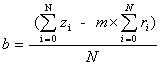The equation used to derive the best fit least square line is stated below:

 For the best fit least square line , the equations are;

where    

                                                z – z-distance value along the log length

                                         - Strip radii

The least square line or average line scheme has to be implemented for all the strip radii in the profile, hence making the approach computationally intensive. Finally the problem with the gaps in the profile was solved using some simple polar filling scheme. Creating polar profile data points in PCS to fill in the gap between data points would resemble the points created by the ellipse fill algorithm in the Dataprocessor module in FCS.

One of the major problems that arise from this new approach is the amount of computation required. The complexity arises from the overhead calculations required to produce the polar profiles. Increasing the processor speed would solve this problem. However, the company wants a solution that will work with the present hardware and hence a different approach had to be taken. The minimum processor speed that satisfies the requirements of the new approach is greater than 1GHz.

2.2.2.3         Halo Filter Technique

The above figure only shows the strip creation for one head. This process is performed on all the heads along the log distance. The halo filter would be inserted into the scanner server right before the scan data points are converted from HCS to FCS. The strip is at present hard-coded to be of 1in length and in the future will be modified to user-defined length.

 The rest of the routine follows the same procedure as the radial strip algorithm, i.e., a an acceptance zone filter of user-defined width along the z-distance is setup to create a LSQ line for each strip and then the strips outside the filter threshold are discarded. The width along the z-distance and the filter threshold can be determined using trail and error technique. There is a necessary tradeoff between the width of the acceptance zone filter and the filter threshold since the smaller the window the smaller the threshold value of the filter has to be to discard the out-of-range data.

 The halo filter technique can be seen to lie between the present approach and the radial strip approach. If the number of strips is set to one then there would only be four scans for each profile and we would face the problems of the present system. If the number of strips is a hundred, then each profile is created by four hundred so-called scans (the four scans from the heads are broken into 100 tiny scans each) resulting in the radial strip approach; thus making the approach computationally intensive.

2.3      Surface Roughness Detection

The next few sub-sections present the solution that I chose from among several approaches to solve the surface roughness detection problem.

2.3.1          Current technique

The current technique used for detecting bumps and depressions uses the perimeter of each profile to determine whether a bump or depression exists.  The perimeter technique computes an average perimeter for the cross-sectional profiles and then uses this information to create a an acceptance zone to flag any cross sectional profiles that deviates from the average perimeter. Depending on the direction of the deviation, the presence of a bump or depression is indicated using the corresponding z-value of the profile. The problem associated with such a technique is that the location of the bump or depression is only given along the log length, i.e. in the z-direction. Another problem associated with this technique is that if a profile contains both a bump and a depression, then the perimeter scheme could fail since the two features together would make the perimeter to contain neither bumps nor depressions while applying the band pass filter. Therefore each profile point must be dealt with individually. Such a scheme would be computationally intensive similar to the profile creation solution.

2.3.2          Some Useful Definitions Related to Detection of Surface Features.

To reiterate certain key points: the image of a log surface is “constructed” from the points obtained by laser scanners. The coordinates of these points have been transformed from the head coordinate system into the log coordinate system. Most of these points represent the actual log surface and its features, but a small percentage of the points are erroneous and do not correspond to the real surface of the log.  All points include imaging and calibration errors. For the subsequent discussion it is also useful to define and discuss the following terms.

2.3.2.1         Underlying shape of the log.

This shape may be thought of as given by the actual surface of the log but with its features, such as bumps, depressions, etc. completely smoothed out. The smoothing process is explained in detail in section 2.3.3.2.

2.3.2.2         Log Axis.

A logical definition of the log axis would be a (smooth) line connecting the center of the underlying shape of the log using only one of the log ends to determine the center and keeping this determined center as the center of the log throughout the log length. However, in our case, the log axis would be a line connecting the centers of the actual shape of the log.  This is because the randomly located surface features, and consequently the line connecting them would affect the coordinates of such centers and would neither be centered nor smooth.

2.3.2.3         ”Chicken-and-the-egg” dilemma:

The generation of the underlying shape of the log requires smoothing of the actual log surface, and it is done with the use of moving averages (long and short) of the strip radii of the actual log surface from the distances from the log axis. Unfortunately the log axis is a (smooth) line connecting the centers of the underlying shape of the log, which we are trying to generate in the first place.

An approach that overcomes this dilemma is to calculate the log axis approximately using an iterative approach described in section 2.2.2.1. Our tests have shown that the log axis defined in this manner works well in determining both the underlying shape of the log and the surface features.

2.3.3          Course of Action

A number of approaches were initially tested including a variation on the perimeter scheme, but none of them accurately located bumps. For example the perimeter approach fails if there is a bump and a depression in the same length location of the log but on opposite sides. Almost all the approaches relied on the profile contours to determine the bumps. The cross-sectional slices individually cannot clearly identify whether a bump exists or not, i.e., using individual profiles to locate a bump or a depression did not succeed because the individual profiles do not have enough information to deal with missing points. Therefore a number of neighboring profiles must be looked at together along the log length for better surface feature recognition. The final approach creates the same radial strips that were used in the radial strip technique for profile creation. It takes a particular strip radius in a profile and follows it along the log length, allowing us to create a line of one particular angular strip radius along the log length.

2.3.3.1         Creation of a Polar Profile

The profile points are converted to polar coordinate values immediately after the entire log is scanned. The polar profiles are then grouped into wedges and a strip radius is found. This step is similar to the radial strip approach.

2.3.3.2         Moving Average – Long and Short

One particular angular strip radius from profiles along the log length is picked and a moving or neighborhood average algorithm is used to create two curves. The first curve is created using the moving average of a short period to represent the true log surface with bumps and depressions somewhat smoothed out. The second curve is created using a longer period to represent the underlying log surface with the bumps and depressions essentially removed. Both these curves must be generated for each particular strip radius location on the log. 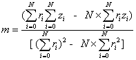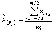The equation of a moving average is stated below:

where

                                          - the window size of the moving average

                                    - Strip radii along the log length at a particular wedge

                            - z-distance value along the log length

3         EXPERIMENTAL ANALYSIS

A detailed analysis of the entire surface feature detection procedure was performed on the scanners. This section provides a methodology for determining the best threshold values for the strips used in the halo filter and window size of both the long and short moving average. Please note that the same test experiments can be performed to detect depressions since bumps and depression are mirror aspect of one another. The accuracy error in bump location and size that are required are given in table 2.

3.1      Bump-Depression threshold determination

This section talks about how the bump and depression threshold values for both the bumps and depressions were determined. Since the threshold value for bumps is similar in magnitude to the threshold of the depressions only the bump threshold is dealt with in this report. Similar results were also obtained for depression thresholds.

 To locate the threshold value of the bumps, we must know the length of the moving averages, both long and short, and also the actual bump height.

3.1.1          Length of moving average – Long and Short

Since the average length of a log is setup at 16ft, we require a long moving average period that would follow the underlying shape of the log. For e.g., if we scan a curved log, the long moving average should smooth a bump whose maximum diameter is 6in yet follow the curve of the log. For an average log length of 16ft, the long moving average period is initially determined to be 2ft. Determining the short moving average period requires two criteria to be met. One is the shortest bump possible and other is the biggest bump possible. We need at least two scans per bump, and since the fastest scan rate is 0.5in/scan, the smallest bump is 1in. Hence the low extreme of the short moving average period is 1in. The largest bump that occurs on a log is approximately 6in. This would set the high extreme of the short moving average at 6in.

3.2      Test case

A number of sample-scans of the log were taken with varying long and short moving averages. The long moving average was kept constant and the short moving average was varied and vice versa.

Keeping the long moving average at 24in (see section 3.1.1) and varying the short average the following results are obtained. The straight lines on the graph represent the error in location while the dotted line represents the error in distance for the angular and Z (along the log length) orientations. A comparison of the error variance in z-location and the z-length of the bumps for different short moving average length were performed and the result is illustrated in figure 14 and 15 respectively.

Using the comparison results from above the best short and long moving average periods for the location of the bumps is 2in and 12in respectively. However, the periods are only applicable for the constraints and the user defined parameters given in table 3 & 4. If the values in these tables were altered then the above comparison procedure has to be performed again to obtain the best moving average periods. The error in the location and the length of the bumps also changes with the change in moving average period. From the figures above it seems that the error variance seems to change linearly with the changes in the moving average period.

3.3        Discussion of Results

As it is evident from the results of the experiment the accuracy of the bump detection is not as good as was expected. However, using the test results we can find that the best values for the long and short moving average in terms of bump detection accuracy is 12in and 2in respectively. The reason for such poor accuracy reading is because the number of strips was limited to 36 strips and hence the interval for the angular location and angular width was 10degrees. By doubling the number of strips, the accuracy of the bump detection doubles but this step slows down the processing speed of the scanner server to greater than twice the current speed.

Another factor that influences the accuracy of bump detection is the halo filter window size. For this experiment the window size was set at 7in. Varying the window size and the halo filter width (stated in table 3) would increase the accuracy of the bump detection but this step would also slow down the processing speed. At present the processing speed of the scanner server with present constraints and specifications is under around 1sec. This value is fine for the test lab environment but must be brought down for field application of the software. Clearly there is more work to be done the scanner server. Some of things that would have to be modified are stated in the conclusion section of this report.

3.4        Accuracy of Bump location and size

The procedure to the experiment is that the log was scanned 10 times with the bump of size stated in table 6 and the result is whether the surface roughness detection feature located the bump. The result was that the probability of locating the bump given the parameter values stated in table 6 was 90%.

After performing such experiments on the new scanner server, it is evident that this is not as long-term solution to the problem. A more clear-cut solution must be implemented and that requires hardware modifications. With the present hardware, the surface roughness feature can only be used to estimate the location of bumps and depressions. Table 7 contains a summary of the design specification for the scanner server and the related values that was obtained by using the surface roughness detection and profile creation technique.

3.5        Runtime Reduction

The addition of the surface roughness detection feature into the scanner server slows the overall performance of the scanner server. Changes must be made to compensate for the additional computational time. The existing scanner server, i.e. the scanner server without the surface roughness feature or the profile creation algorithm, takes approximately a second to scan the log and send the data to the optimizer. The proposed scanner server, i.e., the scanner server with the algorithms present and the number of strip set at 36, takes 5 seconds to scan a log and send the data to the optimizer. However this value will increase at nonlinear rate if the number of strips in the halo filter algorithm and in the surface roughness feature algorithm was increased. The minimum system requirements for the scanner server to work properly have to be upgraded to a Pentium III 200Mhz with 96Mb ram. One option that is always available is to remove the surface roughness feature from the scanner server and implement it inside another software module software, for examples the optimizer. However, this step may increase the processing time of the optimizing software. Or the surface roughness detection feature can be run as independent software.

4         CONCLUSION

My thesis project involved detecting surface roughness features on the log surface and locating the position and size. This information is very important to the sawmill industry since the location of a bump usually means that there is a knot in the log and knots degrade the quality of the wood. Locating bumps and depressions can help to optimize the log cutting process and make appropriate changes to the cutting pattern to compensate for a bump’s presence. The detection of bumps and depressions can also help in grading the quality of lumber products even before the log is sawn, thus increasing the yield of the sawmill and the dollar value per log. Another important use of surface roughness detection is to check if the log was rotated to the correct orientation.

The accuracy of the bump detection algorithm is not as good as expected but this thesis project is a big step in the research undertaken towards the goal of accurately detecting bumps and depressions. The required accuracy for the detection of bumps is less than 0.5in for a log feed rate of 300ft/min, however the accuracy of the proposed bump detection scheme is 5in for a log feed rate of 300ft/min or around 2in for log feed rate of 100ft/min. The accuracy of the surface roughness feature detection algorithm can be improved by number of methods:

It should be noted that that no matter how much you modify the surface roughness feature algorithm in the scanner server, the server’s performance will reach a peak after which improvement will depend on modifying the scanner hardware. Better scanners and faster computers are necessary for more accurate detection of bumps and depressions. At present there is no feedback to the optimizer once a log is turned since there is no reference point to measure the rotation of the log. In the future, surface roughness detection can be used to determine how much the log has actually rotated compared to the desired rotation angle.

                                                                                   ***********

5        REFERENCE

Thomas Block, Best-Fit Circle Algorithm, http://forum.swarthmore.edu/epigone /sci.stat.math/plingkixhix, October 1999.

James Stewart, 1991, Calculus, Second Edition, California: Brooks/Cole Publishing Company.

Jay L. Devore, 1991, Probability and Statistics for Engineering and the Sciences, Third Edition, California: Brooks/Cole Publishing Company.

Ivor Horton, 1997, Beginning Visual C++, Birmingham: Wrox Press Ltd.